Data Storage & Database Systems

In modern application development, choosing the right data storage and database systems is critical. In this blog, we’ll explore core concepts around how data is stored and managed. We’ll compare relational vs. non-relational databases, discuss data modeling and schema design considerations, dive into the CAP theorem and consistency models, and examine indexing, replication, and sharding strategies for scaling.

Relational vs. Non-Relational Databases

Relational databases (SQL databases) and non-relational databases (NoSQL databases) are two broad categories of data stores. Each comes with its own philosophies, strengths, and trade-offs. Let’s break down what they are and how they differ:

• Relational Databases (SQL): These store data in a structured format using tables with rows and columns. Tables can relate to each other via foreign keys, hence the name “relational.” Data is manipulated with Structured Query Language (SQL). Relational databases enforce a rigid schema – you define tables and columns (with data types) upfront, and every row must adhere to that schema. They are known for ACID compliance, meaning they ensure Atomicity, Consistency, Isolation, and Durability of transactions (all-or-nothing transactions, consistent state, isolated concurrent operations, and durable storage of commits)​. Classic examples include PostgreSQL, MySQL, Oracle, and SQL Server.

• Non-Relational Databases (NoSQL): This is an umbrella term for databases that do not use the traditional table schema. They can store data as documents (e.g. JSON documents in MongoDB), key-value pairs (like Redis or DynamoDB), wide-column stores (like Cassandra), or graphs, etc. NoSQL databases typically offer a flexible schema, allowing storage of unstructured or semi-structured data without predefined tables. They often sacrifice some ACID guarantees in favor of scalability and performance, embracing the BASE philosophy (“Basically Available, Soft state, Eventual consistency”). NoSQL systems are designed with horizontal scaling in mind – meaning they can distribute data across many servers more easily than the typically vertically-scaled SQL systems​.

When to choose which? Relational databases shine when data integrity and complex querying (JOINs across multiple tables) are required. They ensure consistency and are ideal for structured data – for example, a banking system where transactions must follow strict rules. Non-relational databases excel for flexibility and scale, especially with big data or fast-changing schemas – for instance, storing JSON configurations, user activity logs, or caching results. Many modern applications actually use a mix: a relational database for core business data and a NoSQL store for specific needs (caching, full-text search, analytics, etc.).

To visualize the difference, consider an example domain: an e-commerce customer and their orders, addresses, product reviews, etc. In a relational model, this data would be normalized into separate tables (Customer, Order, Address, Product, Review), linked by keys. In a document model, all relevant info for a customer might be stored in a single JSON document. Let’s see what that looks like.

Relational data model: information is split into multiple tables (Customer, Order, Address, Product, Reviews), with relationships via primary/foreign keys. Each green box represents a table, and arrows indicate how a customer record links to their orders, addresses, etc. Data is organized in a structured, normalized way, which avoids duplication and ensures consistency across related records​. Queries can join these tables to gather full customer information when needed.

Document-based data model: all information related to a customer (orders, product details, reviews, addresses) is embedded within a single JSON-like document. This denormalized approach stores the customer’s data in one place, which can simplify read operations – one query can fetch the entire customer document without needing multiple JOINs​. The trade-off is potential data duplication (e.g., product details repeated in each order) and more complex updates if, say, a product name changes, since many documents might need modification. However, it aligns well with object-oriented programming (data comes out already aggregated) and can be more natural for certain use cases.

Relational vs. Non-Relational: Practical Example (PostgreSQL vs. MongoDB)

To make this concrete, let’s implement a simple order tracking scenario in both a SQL and a NoSQL database. Our scenario: we have Customers who place Orders. Each Order has a product name and amount. In a relational design (PostgreSQL) we use separate tables and a foreign key; in a document design (MongoDB) we embed orders inside the customer document.

PostgreSQL (Relational) approach: We’ll create two tables – customers and orders – and relate them:

-- PostgreSQL: Define tables
CREATE TABLE customers (
    id SERIAL PRIMARY KEY,
    name TEXT
);
CREATE TABLE orders (
    id SERIAL PRIMARY KEY,
    customer_id INT REFERENCES customers(id),  -- Foreign key to customers
    product TEXT,
    amount INT
);

-- Insert a customer and two orders for that customer
INSERT INTO customers (name) VALUES ('Alice');
-- Assuming the new customer got ID = 1
INSERT INTO orders (customer_id, product, amount) VALUES 
    (1, 'Laptop', 1200),
    (1, 'Mouse', 25);

-- Query: fetch customer info with their orders using a JOIN
SELECT c.name, o.product, o.amount
FROM customers c
JOIN orders o ON o.customer_id = c.id
WHERE c.name = 'Alice';

When we run the SELECT query, the database performs a join between the tables to gather Alice’s orders. The result might look like:

 name  | product | amount 
-------+---------+--------
 Alice | Laptop  | 1200
 Alice | Mouse   |   25

This approach ensures data is normalized (customer info stored once in customers table, orders in orders table). If Alice’s name changes, we update one row. But retrieving all orders requires a join.

MongoDB (Document) approach: We’ll store customer and orders together as one document in a customers collection. Using the Mongo shell (JavaScript syntax):

// MongoDB: Insert a customer document with embedded orders
db.customers.insertOne({
    name: "Alice",
    orders: [
        { product: "Laptop", amount: 1200 },
        { product: "Mouse", amount: 25 }
    ]
});

// Query the customer by name (the orders come along as embedded data)
const alice = db.customers.findOne({ name: "Alice" });
printjson(alice);

The stored document for Alice would resemble:

{
  "_id": ObjectId("..."),
  "name": "Alice",
  "orders": [
    { "product": "Laptop", "amount": 1200 },
    { "product": "Mouse", "amount": 25 }
  ]
}

A single findOne returns Alice’s record with all her orders embedded. There’s no need to join multiple collections in this case, since all relevant data is in one place. This denormalized design makes reads very efficient (one lookup for all data). However, if an order needed to reference a product from a separate collection, or if orders were large in number, we might consider storing them separately or using references. NoSQL allows both embedded documents and references; the choice depends on access patterns (embed if data is usually fetched together, separate if data is reused across many records or frequently updated independently).

Takeaway: Relational vs. non-relational design decisions often come down to joining vs. embedding. SQL uses relations to avoid duplication, while NoSQL may allow duplication to optimize reads. Neither is “better” universally; it depends on the use case. As a developer, consider how your data will be accessed: if you frequently need aggregated data (like a customer and all their info at once), a document model might be simpler. If you need strict consistency and the ability to query data in many ad-hoc ways (filtering, joining on various fields), a relational model is powerful and expressive.

Data Modeling and Schema Design

Data modeling is the process of defining how you structure your data — which entities (tables or documents) you have, what fields they contain, and how they relate. Schema design refers to this structure definition. Good schema design is essential for both correctness and performance. Let’s explore some principles for both relational and non-relational databases:

Relational Modeling & Normalization

In a relational database, schema design often follows the principles of normalization. This means structuring your tables such that each fact is stored only once, minimizing redundancy​

. For example, instead of storing a customer’s address in every order row, you’d have a separate Address table and reference it via an address_id. Normalization (through normal forms like 1NF, 2NF, 3NF, etc.) helps eliminate anomalies when inserting, updating, or deleting data.

The process typically involves:

• Identifying entities (e.g. Customer, Order, Product, etc.) and creating separate tables for each.

• Choosing primary keys for each table (unique identifiers).

• Establishing relationships using foreign keys (e.g. Order table has a foreign key customer_id referencing Customer table).

• Ensuring consistency with constraints (data types, NOT NULL, UNIQUE, etc. to enforce valid data).

The benefit of a well-normalized relational schema is data integrity – you cannot accidentally have mismatched or duplicate info easily. It’s also often easier to update one piece of data (change a product name in one place and all orders reflect it via the join). The downside can be performance on complex queries, since retrieving a complete picture may require multiple JOIN operations across tables. Proper indexing (which we’ll discuss later) and careful query planning mitigate this in many cases.

NoSQL Modeling & Denormalization

Schema design in a NoSQL (document) database is more about optimizing for your query patterns. Since NoSQL allows flexible schema, you can choose to embed or separate data based on what queries you need to run. The common mantra is “design for the use case.” If our application always needs to fetch a user and their recent activity together, putting them in one document makes sense. If two pieces of data are almost always accessed independently, they might go in separate collections.

Key considerations for NoSQL schema design:

• Embedding vs Referencing: To embed or not to embed is a central question. Embedding (nesting sub-documents or arrays) can eliminate the need for joins and make reads very fast (all data in one place)​

  However, embedding can lead to large documents and duplication. Referencing (storing something like a foreign key) keeps data normalized (like a relational model) but then your application might have to do multiple queries (one to get the main document, another to get referenced data) or use $lookup (Mongo’s join-like aggregation) if needed. Generally, embed when data is tightly related and often fetched together; reference when data is reused in many places or frequently updated on its own.

• Schema flexibility: MongoDB does not require all documents in a collection to have the same structure, but having a generally consistent structure is still important for sanity and query efficiency. You don’t explicitly declare a schema, but you should still plan what fields will be present. It’s common to include versioning or migration strategies for documents as your application evolves (since adding a new field won’t break the database, but your code might have to handle missing fields in old docs, etc.).

• Atomicity and transactions: Remember that in many NoSQL databases, operations on a single document are atomic, but multi-document operations are not (unless you use multi-document transactions in MongoDB, which have some limitations). This means if you have a heavily denormalized design (duplicating data), updating that data consistently in many places can be challenging. Sometimes the schema might duplicate read-mostly data but still keep some critical data single-sourced. For instance, you might embed product name and price in an order for quick access, but the authoritative price is in a central product document – if price changes, you might update it in new orders but leave old orders unchanged as a historical record.

Example – Modeling Blog Posts & Comments:

• Relational Schema: A posts table and a comments table, where each comment has a post_id foreign key to its post. To fetch a post with comments, you’d join or do two queries. This is normalized (no duplicate comment data) and each comment is an independent row.

• Document Schema: A posts collection where each post document contains an array of comment sub-documents. Fetching a post with its comments is a single query returning one document. This is denormalized (comments are stored inside a post). Adding a comment means updating the parent post document (which, if comments array grows large, might be less efficient).

There’s no one-size-fits-all answer – the choice depends on scale and access patterns. In a high-throughput system, you might even combine approaches: store data in a normalized SQL database for consistency, and also maintain a denormalized cache or search index for fast reads. The important thing is to think about how your data will be used and design accordingly.

CAP Theorem and Data Consistency Models

When designing distributed database systems, you’ll encounter the famous CAP theorem and various consistency models. Let’s demystify CAP and what consistency means for your app.

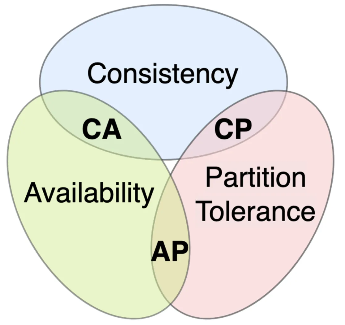
CAP Theorem in a nutshell: CAP stands for Consistency, Availability, Partition tolerance. The theorem (Brewer’s theorem) states that in any distributed data system, you can only guarantee two out of three of these properties​. If a network partition (a break in communication between nodes) occurs, the system has to choose between being consistent or available​

• Consistency (C): Every read receives the most recent write or an error. In other words, all nodes see the same data at the same time​. If you write something and then read it (from any node), you’ll get that write (no stale data). Under partition, a consistent system will refuse reads/writes that can’t be guaranteed (it might return an error rather than stale data).

• Availability (A): Every request receives some (non-error) response, even if some nodes are down​. An available system continues to operate and return responses (possibly older data) despite failures. Under partition, an available system will still process requests, but can’t guarantee those requests see the latest data.

• Partition Tolerance (P): The system continues to work despite arbitrary network partitions​ . This is generally not optional – in a distributed system, network failures will happen, so partition tolerance is usually a given requirement. It means the system can sustain communication breakages between nodes and still function in some capacity.

CAP Theorem Venn Diagram: In a network partition, a distributed system must choose either consistency (CP) or availability (AP). CA (consistency + availability without partition tolerance) is only possible when the system is not distributed or the network is perfectly reliable – a single-node database can be CA since there’s no partition to tolerate. But in a cluster, once a partition occurs, you face a trade-off. For example, a CP system will prefer consistency: it may refuse to serve requests on a partitioned node (sacrificing availability) to avoid serving stale data. An AP system will prefer availability: it continues to serve requests on all nodes (even partitioned ones), accepting that data might not be consistent across nodes until the partition heals.

Most distributed databases are either CP or AP under the presence of partitions​ . Let’s connect this to real databases:

• Traditional SQL databases (when run on a single node or with synchronous replication) lean towards Consistency over Availability​. If they cannot confirm a write on the replicas or the single node is down, they’d rather error out (be unavailable) than allow inconsistent data. For example, a PostgreSQL primary with synchronous replicas: if it can’t reach a replica to replicate a transaction, it may block progress (trading availability for consistency). These systems assume partitions are rare and correctness is paramount. In CAP terms, they tend to be CP in a distributed setup (or CA if you consider a single-node as no partition scenario).

• Many NoSQL databases (especially those designed for distributed scale, like Cassandra or Amazon Dynamo-inspired systems) lean towards Availability over strict consistency. They’ll allow reads/writes on partitioned nodes and reconcile differences later (this is called eventual consistency). For instance, Cassandra is often cited as an AP system: it is designed to always accept writes (to any replica, even if others are down) and gossip the changes to others asynchronously. MongoDB by default (with a single primary-secondary setup) is CP – if the primary is partitioned away from secondaries, it steps down and won’t accept writes until a new primary is elected (so it sacrifices availability briefly to ensure only one primary accepting writes). However, MongoDB can be tuned with write concerns and read preferences to offer tunable consistency — you could choose to read from secondaries (potentially stale, for more availability) or only primary (for consistency). So some databases blur the lines and let you configure how much C vs A you want.

Consistency Models (Strong vs Eventual): Outside of the strict CAP context, in practical terms we talk about how up-to-date the data is on reads in a distributed system:

• Strong Consistency: After you write data, any subsequent read (to any replica) will return that data. This is equivalent to the CAP “consistency” guarantee. It often requires things like quorum writes/reads or single-leader architectures where reads go to the leader. Example: in a strongly consistent system, when Alice posts a comment and immediately refreshes, she always sees her comment. Google’s Spanner (a globally distributed SQL DB) aims for strong consistency across datacenters using TrueTime (GPS-synchronized clocks) to coordinate — this is hard to achieve but they sacrifice latency for it. Most relational databases provide strong consistency on a single node (or within a primary/leader).

• Eventual Consistency: After a write, it’s not guaranteed that immediate reads will see it; however, if no new writes occur, eventually all replicas will converge to the last value. In an eventually consistent system, Alice might post a comment and a read from a different replica immediately after might not show it, but after some seconds, all replicas have it. This model is often acceptable in use cases where slight delays are fine (like social media feeds, where if a comment appears a second later, it’s not the end of the world), and it allows higher availability and partition tolerance. DynamoDB, Cassandra, CouchDB, etc., by default are eventually consistent (though many offer tunable consistency where you can request strong consistency at the cost of latency or availability).

There are also models like “Read-your-writes” consistency, “Monotonic reads”, “Session consistency”, etc., which are nuances ensuring certain user expectations (for instance, read-your-writes is a guarantee that your subsequent reads will reflect your writes, even if globally the system is eventually consistent). These are provided by some systems to make eventual consistency a bit more predictable for users. For example, MongoDB’s drivers by default provide read-your-write consistency on the primary by routing your read after a write to the primary, not a secondary.

The key takeaway for a developer is to understand the consistency needs of your application. Do you absolutely need every read to have the latest data (e.g. bank account balance after a transaction)? If yes, design for strong consistency (CP side of CAP, maybe using a relational DB or a strongly-consistent distributed DB). If your app can tolerate slight delays in propagating updates (e.g. a “like” count that might update a few seconds later), you can choose more AP, eventually-consistent systems that might be more available and partition-tolerant. Often, layering strategies like caching (which might serve slightly stale data) or queueing writes can introduce eventual consistency even if your database is ACID – so it’s always a spectrum and a conscious decision.

Indexing, Replication, and Sharding Strategies

Now that we’ve covered data models and consistency, let’s discuss how to make databases performant and scalable. Three key techniques are indexing (for query performance), replication (for reliability and read scaling), and sharding (for horizontal scaling of write workload and data volume). These are not mutually exclusive – they are often used together in large systems.

Indexing

An index is a data structure that helps speed up data retrieval on specific columns (or fields). In relational databases, an index is often a B-tree (or variants like B+tree) that allows binary search-like efficiency instead of scanning every row. In PostgreSQL, for example, if you query SELECT * FROM orders WHERE customer_id = 123;, having an index on orders(customer_id) means the database can jump directly to the entries for customer 123 instead of reading the entire orders table. This can make a huge difference: without an index, the database does a sequential scan through potentially millions of rows​ with an index, it performs a much faster lookup, resulting in millisecond-range query times even on large tables​.

Creating an index in SQL is straightforward. For example, to index the customer_id in the orders table:

CREATE INDEX idx_orders_customer ON orders(customer_id);

After this, queries filtering by customer_id will use the index to find matching rows quickly. Behind the scenes, PostgreSQL maintains the index as data is inserted/updated (which does add some overhead to writes, since the index needs updating too).

NoSQL databases like MongoDB also support indexes. In Mongo, you’d do:

db.orders.createIndex({ customer_id: 1 });

This creates an index on the customer_id field in the orders collection (the 1 indicates ascending order index). MongoDB’s query engine will use this index for queries like find({customer_id: 123}). In fact, indexing in Mongo is very similar conceptually to SQL – it even uses B-trees by default.

When to index: You generally add indexes on fields that are frequently used in query filters, join conditions, or sorting. A primary key is usually indexed by default (ensuring fast lookup by ID). Be careful not to over-index: each index consumes disk space and slows down writes. It’s a trade-off: more indexes = faster reads (queries), but slower inserts/updates and more storage usage. Use tools like EXPLAIN in PostgreSQL to see if a query is using an index or not, and profile your database workload to decide which indexes truly help.

Example: If we often query orders by product name, an index on orders(product) makes sense. But if we never query by amount, an index on amount would be unnecessary overhead. In practice, start with indexes on key search fields and primary keys, then monitor and add indexes as needed for slow queries.

Replication

Database replication means keeping copies of your data on multiple nodes (servers). The most common form is master-slave (primary-secondary) replication: one primary node receives all writes, and one or more secondary nodes replicate those changes (usually asynchronously, but can be synchronous) and are used for reads or standby. The motives for replication are: high availability (if the primary goes down, a secondary can take over) and read scaling (many reads can be spread across replicas, reducing load on the primary).

In PostgreSQL, replication can be set up so that you have one primary and multiple read replicas. The primary logs all changes (WAL – write-ahead log), and replicas continuously apply those logs. If the primary fails, you can promote a replica to become the new primary. Many cloud setups (Amazon RDS, etc.) automate this failover. From a developer perspective, you might connect your app to the primary for writes and to a replica for read-heavy endpoints. Keep in mind replication lag – there’s typically a small delay, so a replica might be a few seconds behind the primary. This is usually fine for eventually-consistent reads (e.g., an analytics query or reading someone else’s updates slightly behind real-time), but not for, say, reading your own recent write (which is why many frameworks allow read-after-write on primary to ensure consistency for that user’s action).

MongoDB’s approach is built-in via replica sets. A Mongo replica set consists of one primary and N secondaries. The driver (client library) will automatically send writes to primary and distribute reads (if you configure it to use secondary reads). MongoDB will handle automatic failover – if primary dies, secondaries elect a new primary among themselves. Mongo’s replication is usually asynchronous (primary writes, secondaries catch up), so it’s also eventually consistent for secondary reads.

Benefits of Replication:

• Fault tolerance: If one node goes down, the data is still available on others (no single point of failure).

• Scaling reads: You can have, say, 5 replicas and handle 5x the read queries (approximately) by load-balancing reads. This is great for read-heavy workloads.

• Geographical distribution: You can place replicas in different regions (e.g., one in US, one in Europe) so that local users get faster read access from a nearby replica. Writes still go to primary (which might be in one region), but reads can be served locally.

Trade-offs:

• Replication doesn’t help write throughput, since every write still has to go through the single primary (vertical scaling or sharding is needed for write-scaling).

• There is complexity in ensuring all replicas are consistent and dealing with lag. If a replica is slow or network is partitioned, it might fall behind. If it’s too far behind, it might be automatically taken out of rotation until caught up (to avoid serving very stale data).

• Writing to multiple replicas (multi-master replication) is another approach (like MySQL NDB Cluster or some multi-primary NoSQL systems), but those introduce conflict resolution issues. Most setups use one primary at a time to avoid write conflicts.

From a developer viewpoint, once replication is set up, you mostly just need to be aware of any lag if your reads go to replicas. Some ORMs or query routers allow specifying read-preference (primary vs replica). For instance, in a Node.js app with Mongo, you can do readPreference=secondaryPreferred for certain queries that can tolerate eventual consistency.

Sharding (Partitioning)

Sharding is the technique of partitioning your data across multiple servers so that each server (shard) holds only a subset of the total data. If replication is about copies for redundancy, sharding is about slices for scalability. Each shard is often a replica set in itself in modern systems (so you shard for scale and also replicate each shard for resilience – these can be combined)​.

There are different strategies for sharding:

• Key-based (Hash) Sharding: You choose a shard key (like user_id, or some hash of an identifier) and use a hash function to distribute records across shards. For example, with 4 shards, user_id 1000-1999 might go to shard1, 2000-2999 to shard2, etc., or a hash mod 4 of the key decides the shard. This aims to evenly distribute data. MongoDB lets you specify a shard key on a collection, and it will split data into chunks and distribute across shards.

• Range Sharding: Each shard holds a continuous range of the data. For instance, shard1 has IDs 1-1,000,000, shard2 has 1,000,001-2,000,000, etc. Range sharding can be efficient for range queries (e.g., dates), but if the data or access is skewed (say most new data goes to the highest range), one shard can become a hotspot.

• Geographic or Attribute-based Partitioning: Sometimes you shard by a particular attribute, like region. For example, user records might be partitioned such that European users are on a Europe shard, American users on US shard. This can reduce latency for users and comply with data residency, but it’s essentially a manual partition by a field.

Sharding addresses the limitation of a single machine’s resources. If your dataset is 10 TB, far too large for one server’s disk or memory, you can shard it into 10 machines with 1 TB each. Similarly, if you need to handle 100k writes per second, you can divide the load among multiple shards (10k/sec each, for instance).

MongoDB Sharding: In MongoDB’s architecture, there is a component called mongos (router) that knows how to route queries to the correct shard. The data is partitioned by shard key, and a config server keeps metadata of which chunk of data lives where​.

Each shard is typically a replica set (to have both sharding and replication)​.

So a production Mongo cluster might have: config servers, query routers (mongos instances), and multiple shards (each shard = primary + secondaries). When the application queries Mongo, it goes through mongos which forwards the query to the appropriate shard(s). If you query by the shard key, it can go to the specific shard that has that key. If you do a broad query not keyed by the shard key, the router may broadcast it to all shards and aggregate results (which is slower). So designing a good shard key that evenly distributes data and matches your common query patterns is crucial.

Sharding in SQL: Traditional SQL databases were not trivially sharded – they assumed one big machine. However, modern approaches and extensions exist: for example, PostgreSQL can be sharded using table partitioning (which is more manual) or solutions like Citus (an extension that distributes PostgreSQL across nodes). In these, you often pick a distribution key for a table, and the system splits data into shards stored on different nodes. There’s no built-in query router in vanilla Postgres, but Citus provides one, or you handle it at the application level. There are also frameworks and proxies (like Vitess for MySQL) that handle sharding behind the scenes for SQL. The takeaway is: it’s doable, but not as out-of-the-box as with many NoSQL systems that assumed sharding from day one.

Challenges with Sharding:

• Complexity: You now operate a cluster of databases instead of one. Monitoring, backups, and operations are more involved.

• Rebalancing: If one shard becomes too full or hot, you might need to reshard or add more shards. Moving data between shards (rebalancing) can be tricky and time-consuming. MongoDB auto-balances chunks across shards, but in some systems you have to do manual data migrations.

• Joins and Transactions: In a sharded environment, cross-shard joins or multi-shard transactions are hard. If your query needs data from two shards, the system (or your application) must gather from both and combine. Some databases support distributed transactions across shards, but it can be slow or limited. Often, schemas in sharded systems are designed to avoid the need for cross-shard operations (e.g., choosing a shard key that groups related data likely to be accessed together on the same shard).

• Partition tolerance vs. consistency: With shards, if a shard (or its network) is unreachable, part of your data is unavailable. The system might choose to still operate with remaining shards (meaning some data can’t be fetched until that shard is back). If high availability is needed, each shard should be replicated (so that a single node failure in that shard doesn’t make the shard unavailable).

To sum up, replication is about copying data for reliability and read throughput, while sharding is about splitting data for capacity and write/read scaling. They solve different problems and are often used together: you might shard a huge dataset across 10 servers, and also replicate each shard to another server for backup. That gives you horizontal scale and high availability (this is essentially how large cloud databases operate).

Designing a High-Read System with Caching and Replication

Finally, let’s put some of these pieces together. Imagine you’re designing a system that is read-heavy – for example, a product catalog API that gets 100 reads for every 1 write, or a popular blog site where content is written once but read many times. Such a scenario calls for optimizations to handle a high volume of read traffic efficiently. Two common strategies are caching and replication. We’ve covered replication; now we introduce caching (with Redis) and outline a design that leverages both.

The Power of Caching (Redis)

A cache is a high-speed data store (often in-memory) that sits between your application and the primary database. Redis is a popular open-source in-memory data store often used as a cache. The idea is to store frequently accessed data in Redis so that subsequent requests can get it from memory quickly, without hitting the slower disk-based database each time. Caching can drastically reduce latency for repetitive reads and reduce load on your database.

Cache-Aside Pattern (Lazy Loading): The most common caching strategy is called cache-aside​

. The application checks the cache first when a read request comes in:

1. Cache hit: If the data is found in the cache, return it immediately – the database is bypassed, which is a big win for performance.

2. Cache miss: If the data is not in the cache, then query the database (this will be slower, but it’s only on a miss). Then populate the cache with that result, so that next time it will be a hit​. Finally, return the data to the user.

By doing this, you ensure that data which is frequently requested ends up being served from the fast cache after the first miss. Less-frequently accessed data might not be in cache, but that’s okay – you only pay the cost on those infrequent requests.

Let’s illustrate this in code with a simple example using Redis (in pseudocode/Python for clarity):

import redis
r = redis.Redis(...configure connection...)  # connect to Redis

def get_product_details(product_id):
    cache_key = f"product:{product_id}"
    # 1. Try cache first
    cached_data = r.get(cache_key)
    if cached_data:
        # Cache hit
        return deserialize(cached_data)

    # 2. Cache miss: query the primary database (e.g., PostgreSQL)
    product = db_query_product_by_id(product_id)
    
    # Store the result in cache for next time, with an expiration time for safety
    r.set(cache_key, serialize(product), ex=300)
    return product

In this snippet, db_query_product_by_id represents the call to your database to fetch the product info. We then store it in Redis with a key like "product:1234" and perhaps set an expiration time (TTL) of 5 minutes (300 seconds) to avoid keeping stale data forever. The next call within 5 minutes will find it in Redis and skip the database.

Cache invalidation: One tricky aspect with caches is keeping them in sync with the database. If the underlying data changes (say, a product price is updated), the cache might serve old data until it’s refreshed or expired. Strategies to handle this include:

• Setting a reasonable TTL (time-to-live) on cache entries so they expire and get reloaded periodically (as done above).

• Proactively invalidating or updating the cache when a write happens. For example, after updating the product price in the DB, you could DEL product:1234 from Redis or update it with the new value. This requires your application to have hooks on writes to clear the relevant cache keys (write-through or write-behind caching strategies​).

• In some scenarios, it’s acceptable that stale data is shown for a short time (like a few seconds) – this is the price for extreme read efficiency. For instance, a count of likes might lag slightly behind the actual count. Each system must decide the tolerance for staleness.

Redis as a cache is super fast (in-memory operations, often completing in <1 millisecond). It can handle hundreds of thousands of ops per second easily. By offloading frequent reads to Redis, your primary database is freed up to handle writes or less frequent complex queries.

High-Read Architecture: Combining Replication and Caching

For a high-read, moderately-write system, here’s a common architecture that uses both replication and caching:

• Primary Database (PostgreSQL): This is the source of truth. All writes (inserts, updates) go here. The primary might also handle some reads, but we aim to reduce its load.

• Read Replicas: We set up one or more replicas of the Postgres primary. These replicas continuously apply the primary’s changes. Our application can direct read-only queries to these replicas. For example, analytical queries or any endpoints that are read-heavy and can tolerate slight replication lag go to a replica. This immediately multiplies read capacity (if you have 3 replicas, you roughly quadruple read throughput assuming even distribution including primary).

• Redis Cache Layer: In front of the database queries, we incorporate Redis as described. The application first checks Redis for cached results. We might cache the results of specific expensive queries or the output of constructing API responses. For example, if users frequently request the “top 10 products” list, that could be cached. Or each product detail could be cached individually as we showed. The cache can store fully rendered JSON responses or just database query results, depending on the use case.

How a request flows: When a user’s request comes in for data, the application does: check Redis -> if miss, query a database (possibly a read replica) -> then store result in Redis -> return to user. By doing this, if the same or another user hits the same endpoint again, the data comes straight from cache.

If the data is not found in cache and we go to the DB, ideally we hit a read replica (so the primary isn’t burdened). The read replica returns the data (slightly slower than cache but still typically on the order of tens of milliseconds), then we cache it. If the data was recently updated, there’s a small chance the replica hasn’t got the latest write yet (replication lag). In such cases, we might momentarily serve slightly stale data. Depending on requirements, one could choose to always read from primary when caching (to ensure freshest data in cache), or one could accept eventual consistency. Often, critical reads (after a recent write that the user is expecting to see) are directed to primary, and more generic reads go to replica.

Scaling out: This combination of caching and replication can handle very large read volumes. The cache handles the hottest data almost entirely in memory. The replicas handle other read traffic in parallel. The primary handles the writes. You can add more replicas if read load grows (horizontal scaling for reads). You can also scale the Redis cluster if needed (Redis itself can be clustered or just use a stronger box).

Use case example: Think of Twitter’s timeline. Each user’s home feed could be cached (so if they refresh, it’s not regenerated each time from scratch). The primary database stores tweets, and there are read replicas to serve timelines or search queries. Redis might store the timeline for a short period so that if the user refreshes within, say, 30 seconds, it doesn’t hit the database again. They also use other caching like Memcached. This general idea pops up everywhere high scale is needed: Cache what you can in memory, replicate your data for read throughput, and reserve the main database for the heavy lifting that only it can do (like maintaining consistency on writes).

Important considerations:

• Ensure cache consistency to a level your application needs (through TTL or invalidation on writes).

• Monitor cache hit rates. A low hit rate means either you’re caching the wrong things or the TTL is too low or the cache is too small. You want a high hit rate (e.g., >90%) for the cache to be really effective for hot data.

• For replication, monitor lag. If lag grows (maybe the replica is falling behind due to heavy load), you might need to beef up replica hardware or add another replica to share load.

• Have a strategy for failover: if the primary DB dies, one of the replicas should take over (this can be set up with automatic failover). Also, if Redis cache fails (it’s usually in-memory and not as durable, though Redis can be made persistent or clustered), your system should still function (just a bit slower). Essentially, the system should be resilient: any single component failure should not take the whole system down. The combination of replication and caching helps here – cache is usually non-critical (a luxury that if down, just means queries go to DB), and replication provides backups for the DB.

In summary, a high-read architecture will serve most reads from fast, scalable sources: first the cache (fastest), then replicas (fast and scalable), and lastly fall back to primary if needed. Writes go to primary and propagate out. This design can handle dramatically more traffic than a single database server alone​, and it’s a common blueprint for web applications, APIs, and microservices in the real world. By mastering these strategies – caching frequently accessed data, replicating databases, and sharding when data grows – you as a developer can ensure your application’s data layer is robust, scalable, and performant.

Conclusion

In this blog, we covered a lot of ground in data storage and database systems. We contrasted relational vs. non-relational databases, learning how SQL databases enforce schemas and relationships while NoSQL offers flexibility and horizontal scale. We saw how data modeling differs between the two paradigms, with normalization in SQL and use-case-driven schema in NoSQL (embedding vs. referencing). We clarified the CAP theorem, explaining why distributed systems can’t have it all and how that leads to different consistency models like strong and eventual consistency. We also delved into practical scaling techniques – using indexes to speed up queries, replication to distribute load and ensure high availability, and sharding to partition data across servers for massive scale. Finally, we put it all together in a scenario designing a high-read system with Redis caching and replicated databases, demonstrating how these concepts play out in a real-world architecture.

The key takeaway is that database design is not one-size-fits-all. Each decision – SQL vs NoSQL, how to model data, how to ensure consistency, where to add indexes, whether to replicate or shard – depends on the application’s requirements and usage patterns. As you gain experience, these become tools in your toolbox. Need flexibility and quick iteration? Maybe start with a schemaless store. Need absolute consistency for transactions? A relational database with strong ACID guarantees is the way. Scaling reads? Add caching and replicas. Huge scale writes? Shard the data.

Remember, a well-chosen and well-tuned database strategy can make the difference between a snappy app and one that crumbles under load. Happy coding, and may your queries be ever fast and your systems ever scalable!

References:

• Relational vs. Non-Relational fundamentals​

  mongodb.com

• Advantages of document model and horizontal scaling​

  mongodb.com

• ACID transactions and relational guarantees​

  mongodb.com

• Relational schema example (customer, order, etc.)​

  mongodb.com

• CAP theorem definitions and trade-offs​

  en.wikipedia.org

• RDBMS vs NoSQL consistency (ACID vs BASE)​

  en.wikipedia.org

• Indexing benefits for query performance​

  geeksforgeeks.org

• Replication and sharding explained​

  ltbatis.medium.com

• Combined replication and sharding in practice​

  dev.to

• Cache-aside pattern steps​

  docs.aws.amazon.com